You can find the code for this raytracer here.

How Rays are Cast

The raytracer uses a camera model to cast rays into the scene. For each pixel in the output image, one or more rays are generated and traced through the scene.

Camera setup:

• The camera is defined by its position, look-at point, up vector, and field of view.
• A view plane is calculated based on the camera's properties and the image dimensions.

Ray generation:

• For each pixel, a ray is created from the camera position through the corresponding point on the view plane.
• If jittering is enabled, multiple rays are generated per pixel with slight random offsets for anti-aliasing.

Ray tracing:

• Each ray is tested for intersection with all objects in the scene.
• The closest intersection point is determined.
• Lighting calculations are performed at the intersection point.

Pseudocode for ray generation:

def generate_rays(self):
    for y in range(self.height):
        for x in range(self.width):
            ray = self.generate_ray(x, y)
            self.rays.append(ray)

Geometry and Collision Detection

The raytracer supports primitive and complex shapes. Each geometry type implements its own intersection method.

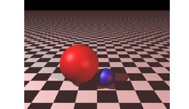
Sphere Collision

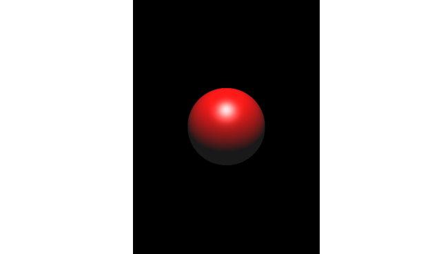
Sphere intersection is one of the simplest and most efficient to calculate. Steps:

1. Compute the discriminant of the quadratic formed by the ray and sphere.
2. If the discriminant is negative, there's no intersection.
3. If positive, calculate the intersection points and choose the nearest one in front of the ray origin.

def sphere_intersect(ray, sphere):
    L = ray.origin - sphere.center
    a = dot(ray.direction, ray.direction)
    b = 2 * dot(ray.direction, L)
    c = dot(L, L) - sphere.radius**2
    discriminant = b**2 - 4*a*c

    if discriminant < 0:
        return False

    t = (-b - sqrt(discriminant)) / (2*a)
    if t > 0:
        return t
    return False

The raytracer supports motion blur effects for moving spheres.

Box Collision (AABB)

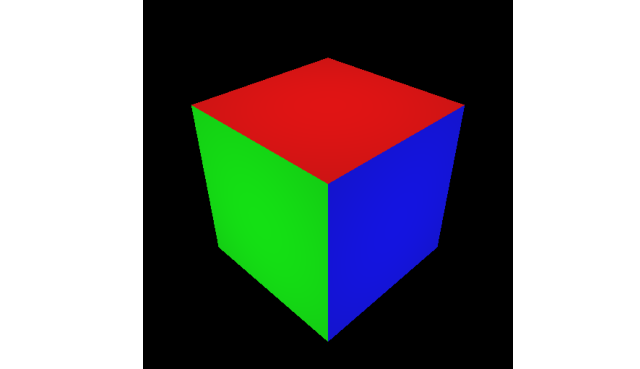
Axis-Aligned Bounding Box (AABB) intersection is implemented using the slab method:

1. Calculate intersections with each pair of parallel planes defined by the box.
2. Find the latest entry point and earliest exit point across all dimensions.
3. If the entry point is before the exit point and the exit point is positive, there's an intersection.

def aabb_intersect(ray, aabb):
    t_min = (aabb.min - ray.origin) / ray.direction
    t_max = (aabb.max - ray.origin) / ray.direction
    t1 = min(t_min, t_max)
    t2 = max(t_min, t_max)
    t_near = max(t1.x, t1.y, t1.z)
    t_far = min(t2.x, t2.y, t2.z)

    if t_near <= t_far and t_far > 0:
        return t_near
    return False

Plane Collision

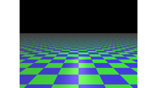
Plane intersection method:

1. Calculate the denominator (dot product of plane normal and ray direction).
2. If the denominator is near zero, the ray is parallel to the plane.
3. Otherwise, calculate the intersection point and check if it's in front of the ray origin.

def plane_intersect(ray, plane):
    denominator = dot(ray.direction, plane.normal)
    if abs(denominator) < 1e-6:
        return False
    t = dot(plane.point - ray.origin, plane.normal) / denominator

Meshes

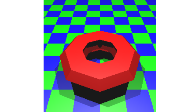
Mesh intersection involves testing against each triangle in the mesh:

1. For each face in the mesh: perform a ray-triangle intersection test.
2. Use barycentric coordinates to determine if the intersection point is inside the triangle.
3. Keep track of the nearest intersection point.

This method can be computationally expensive for complex meshes, so bounding volume hierarchies can be used to optimize the ray-tracing process (as demonstrated above).

Shadows

Shadows are made by casting secondary rays from intersection points towards light sources. If an object blocks the path to a light source, that point is considered to be in shadow.

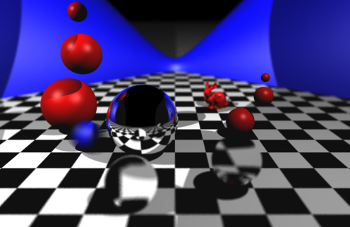
Reflection

Reflection is handled by generating new rays at intersection points where the material is reflective. The direction of these reflected rays is calculated using the law of reflection:

def reflect(direction, normal):
    return direction - 2 * dot(direction, normal) * normal

When a reflective surface is encountered, a new ray is cast in the reflected direction, and the color from this reflected ray is combined with the local color of the object.

Refraction

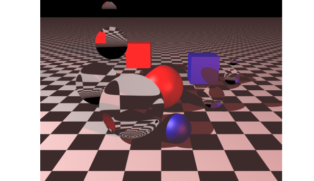
Refraction occurs when a ray passes through a transparent material with a different refractive index. I found this post useful for understanding.

The process:

1. Calculate the angle of refraction based on the incident angle and the refractive indices of the materials.
2. Determine if total internal reflection occurs.
3. Generate new ray in the refracted direction.
4. Trace refracted ray through the scene.

The calc_refracting_ray method handles the complex calculations required for accurate refraction, including handling cases of total internal reflection (introducing an upper limit to the depth of a ray).

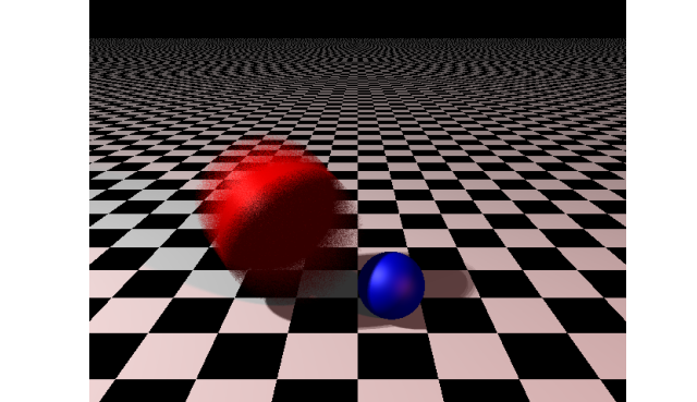
Antialiasing

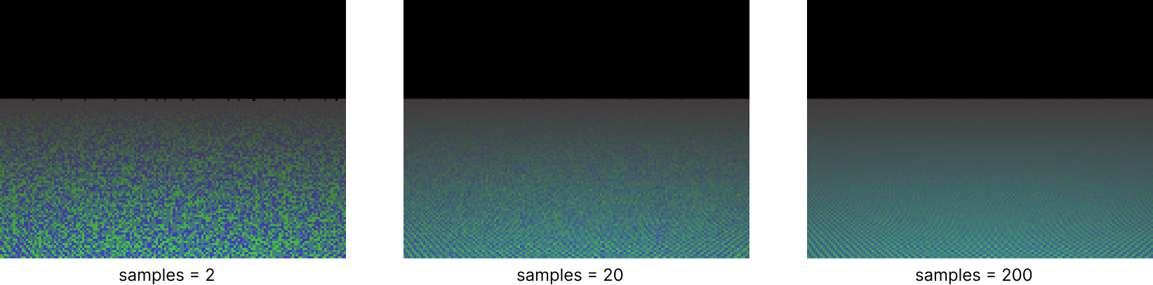
Antialiasing helps reduce the jagged edges (aliasing artifacts) that appear in rendered images, especially along the boundaries of objects or in areas with high contrast.

Implementation:

1. For each pixel, multiple rays are cast with slight offsets, at random.

   if self.jitter:
       random_i = i + random.random()
       random_j = j + random.random()
   else:
       random_i = i
       random_j = j
   

2. These jittered rays are used to sample the scene at slightly different positions within the pixel's area.
3. The results from these multiple samples are averaged to produce the final color for the pixel:

   for _ in range(self.samples):
       ray = self.generate_ray(i, j, left, right, top, bottom, u, v, w, d)
       colour += self.trace_ray(ray)
   colour /= self.samples  # Average the color
   

This is just one possible technique.

Extra

Motion Blur

Motion blur simulates the effect of movement during the camera's exposure time. It's effective for fast-moving objects or rapid camera movement.

How to:

1. Each ray is assigned a random time value within the exposure interval (e.g., 0.0 to 0.2).
2. Moving objects interpolate their position based on this time value.

For spheres, the center position is interpolated:

def sphere_intersect(ray, sphere):
    # ...
    center = sphere.center + sphere.velocity \* ray.time # Use interpolated center
    # ...

The final color of a pixel is the average of multiple samples taken at different times.

This approach creates a realistic motion blur effect, with fast-moving objects appearing smeared in the direction of their movement.

Depth of Field Blur

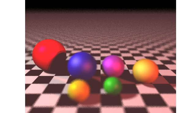
Depth of field (DoF) simulates the focus properties of physical camera lenses, where objects at a certain distance are in sharp focus while objects closer or farther appear blurred.

How to:

1. Define an aperture size and a focal distance.

2. For each pixel, generate multiple rays with origins slightly offset on the camera lens plane:

   def generate_ray(i, j, left, right, top, bottom, u, v, w, d):
   
       if self.dof:
           rd = self.aperture / 2 * self.random_in_unit_disk()
           offset = u * rd[0] + v * rd[1]
           focus_point = self.position + self.focus_dist * ray_dir
           ray_origin = self.position + offset
           ray_dir = glm.normalize(focus_point - ray_origin)
       else:
           ray_origin = self.position
   
       return hc.Ray(ray_origin, ray_dir, ray_time)
   
   

   The random_in_unit_disk() function generates random points within a unit disk:

   def random_in_unit_disk(self):
       while True:
           p = np.array([random.uniform(-1, 1), random.uniform(-1, 1), 0])
           if np.dot(p, p) < 1:
               return p
   
   

3. Trace multiple rays for each pixel and average the results.

This creates a realistic depth of field effect:

• Objects at focal distance remain sharp.
• Objects closer or farther than focal distance become progressively blurred.
• The size of the aperture controls the amount of blur (larger aperture = more blur).

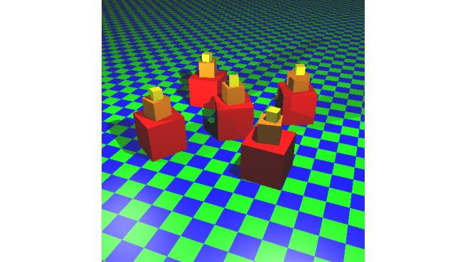
Novel scene

Conclusion

This raytracer demonstrates the power of creating realistic images with a simpe set of rules. With further development, procedures to handle HDR mapping, soft shadows, UV mapping and more can be implemented.